All About Robotic Actuators

Scope

Basically all robot learning embodiments use

• Brushless DC motors (BLDC) (anything by Unitree, Boston Dynamics, I2T’s YAM)
• URs and Frankas use permanent magnet synchronous motors (PMSM)

This is the scope of the paper. I don’t cover dynamixel, hobby servo, or stepper motors which are common in simpler robots. The depth is tuned to be suitable for robot learning practitioners.

Contents:

• Starting from the fundamentals
• Computing Torque:
• Simulating Your Own Actuators in Mujoco

Starting from the fundamentals

All motors can only be controlled by changing the voltage supplied to it

All the motors we care about control voltage with Pulse Width Modulation (PWM). Here’s an example: we can switch a 24V power supply on and off incredibly fast to simulate any voltage we want. If the supply is on 25% of the time, the motor will operate as if it’s supplied with a constant 6V.

PWM executes arbitrary voltages, but it doesn’t know how to control motor speed or torque. This is where Field Oriented Control (FOC) comes in. FOC can calculate the exact voltage the circuit will need in order to get a desired torque. It does so by reading the angle of the motor in order to understand the magnetic cycles of the motor.

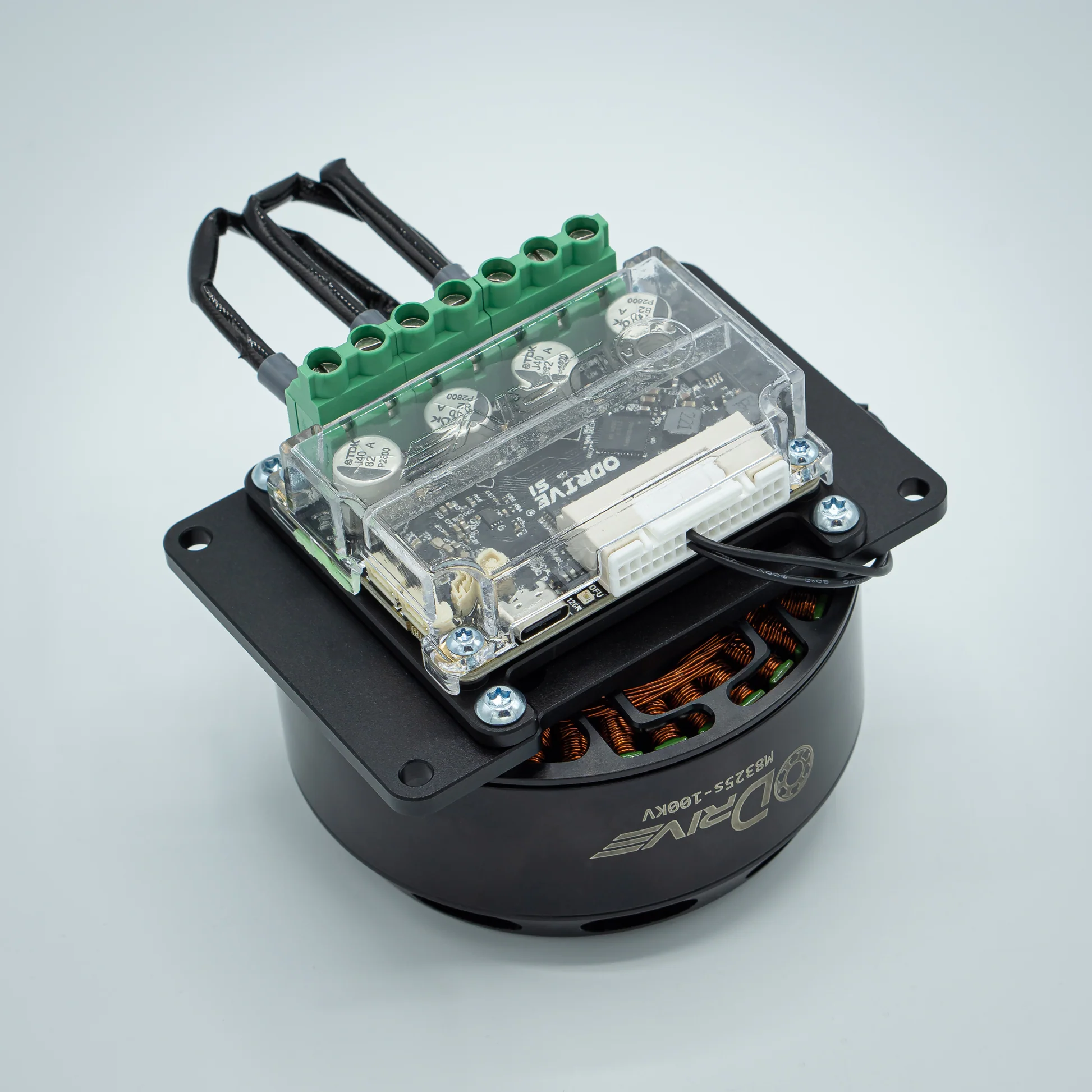
The ODrive S1 is the motor driver most homemade robots use.

With a motor driver, we now only need to worry about torque that we’re sending to the motor driver.

Computing Torque:

Now we need to figure out how to compute the torque command from whatever the neural network outputs. Usually this is a joint position. This is important to understand as we need to simulate this conversion process in low level robot firmware and simulators.

To my knowledge there’s only one paper about learning torque features directly in a policy.

Everyone else has a policy that just learns target joint positions and have either a deterministic equation or a network that maps joint positions to joint torques.

1. Learned Network

This is basically necessary if you work on the Anymal robots, which use highly complicated SEA actuators. But of course any actuator could benefit from using neural networks to learn hard to model dynamics in an actuator.

We can just straight up make a neural network learn torque commands like in this classic paper. They had a dedicated neural network that mapped joint positions to actuator torques, and it was trained on real data collected on the actuator to pick up on signal delays, bandwidth limits (actuators can only react to signals up to a certain frequency), and other non-linear mechanical properties associated with SEA actuators.

Benefits from the paper:

• No gain tuning
• Reduced tracking errors
• Full use of motor capabilities
• It uses energy more effectively
• Better posture when quadruped is walking

Implementation Notes:

• Network needs to update at 200 Hz or more

2. Proportional Derivative (PD) Control

There are two ways to do PD control. Parallel or Nested.

How to tune PD controllers:

Gains depend on the controller frequency: \(K_p\) and \(K_d\) are software-defined numbers. If your high-level ROS 2 node runs at 100 Hz, your gains will have to be completely different than if you are running a tight hardware real-time loop at 1,000 Hz.

• This is why you need to tune the \(K_p\) and \(K_d\) both in sim and in the real world.

Tuning Method

Before you start, ensure the robot is in a safe position and set all gains to zero (\(K_p = 0\), \(K_d = 0\)).

For Mujoco Folks:

• The gains are already tuned for Mujoco Menagerie assets: The default \(K_p\) (stiffness) and \(K_d\) (damping) values inside the <actuator> tags.

For Unitree Folks:

When deploying using unitree_rl_lab (which relies on Unitree’s Low-Level SDK), the firmware sends a continuous stream of motor commands containing 5 main arguments for each joint: q (position), dq (velocity), Kp, Kd, and tau.

How the firmware sets these constants depends entirely on your training paradigm:

For UR arm folks

When using servoJ, the gains are already fundamentally tuned by Universal Robots. The parameter gain=300 that you pass into the function isn’t a custom \(K_p\) or \(K_d\) value that you have to guess from scratch; it is a high-level multiplier that tells UR’s incredibly sophisticated, pre-tuned factory internal loops how aggressively to track your target.

Parameter Breakdown for servoJ

rtde_c.servoJ(q, velocity, acceleration, dt, lookahead_time, gain)

• q (list of 6 floats): The target joint positions in radians. If your neural network outputs position deltas, you must add them to the current actual positions before passing them here.
• velocity (float): The maximum joint velocity limit (\(\text{rad/s}\)). Note: This parameter is largely ignored by the internal controller during real-time servoJ execution, but it must be populated as a baseline safety limit.
• acceleration (float): The maximum joint acceleration limit (\(\text{rad/s}^2\)). Like velocity, this acts primarily as a safety guardrail.
• dt (float): The time step of your control loop in seconds. For UR e-Series arms, this must match the \(500\text{ Hz}\) hardware clock exactly (0.002). For older CB3 arms running at \(125\text{ Hz}\), this must be 0.008.
• lookahead_time (float): The lookahead time in seconds used to smooth the trajectory. Range is typically 0.03 to 0.2. A low value makes the arm highly responsive but jerky; a high value introduces latency but smooths out noisy neural network outputs.
• gain (float): The proportional gain multiplier for the internal position loop. Range is typically 100 to 2000. This parameter controls how aggressively the arm tries to snap to your target position q using its own internal, factory-calibrated stiffness curves.

By default, leaving gain=300 and lookahead_time=0.03 works perfectly for almost every robot learning policy because UR handles the underlying hardware constraints automatically.

Simulating Your Own Actuators in Mujoco

Most popular embodiments are already simulated in Mujoco Menagerie. This part is for people who want to deeply understand what’s going on or rig their own custom robots.

Assuming you know how bodies work in Mujoco, let’s look at the simplest example of an actuator:

import time
import mujoco
import mujoco.viewer

XML = """
<mujoco>
	<worldbody>
		<body pos="0 0 0">
			<joint name="hinge" type="hinge" axis="0 0 1"/>
			<geom type="capsule" fromto="0 0 0 0.3 0 0" size="0.03"/>
		</body>
	</worldbody>
	
	<actuator>
		<motor name="motor" joint="hinge"/>
	</actuator>
</mujoco>
"""

model = mujoco.MjModel.from_xml_string(XML) # compile XML -> mjModel
data = mujoco.MjData(model) # the state (qpos, qvel, ctrl, ...)

# For a <motor>, force = ctrl. So ctrl is the torque applied about the hinge axis.
# Constant torque -> the hinge keeps accelerating (open loop, no feedback).
data.ctrl[0] = 0.05 # constant 0.05 N*m

with mujoco.viewer.launch_passive(model, data) as viewer:
    while viewer.is_running():
        step_start = time.time()
        mujoco.mj_step(model, data)
        viewer.sync()
        dt = model.opt.timestep - (time.time() - step_start)
        if dt > 0:
            time.sleep(dt)

As you can see, to apply an actuator in an XML, just add actuator after world body. Then assign a joint to it.

Here are all of the field in <motor>:

• joint: “hinge” will make data.ctrl use Nm and “slider” will use N
• gear: the gear ratio which affects torque, velocity, reflected inertia…
• armature: the motor rotor’s inertia. Mujoco reflects it through the gear and adds it to the joint inertia, so you pass the raw rotor inertia, not the already-reflected value.
  • Note that this is really important to model correctly with high gear ratio set ups since \(I_{reflected} = I_{rotor} · N_{gear~ratio}^2\), and Mujoco applies the \(N^2\) for you.
• ctrlrange: clamps data.ctrl before actuator force is computed. A command limit.
• forcerange: clamps the scalar data.actuator_force after

Other notes:

<compiler autolimits="true"/>

• Make sure this is set at the beginning to actually apply any limits

Control loops for motors

You can set your control loop to be external to Mujoco, in which case the actuator would just reflect commanded torque. Or, you can set a control loop in Mujoco.